
Share this article
A Hundred Years of the Return Period and the Hundred-Year Flood
A century ago, engineers faced a deceptively simple question: how high should a dike be built to survive a flood that strikes once every hundred years? Out of that question grew an entire statistical apparatus — the return period, the assumption of stationarity, extreme value theory — tools that finance later borrowed, often without acknowledging their origin. Before turning to how this machinery was transplanted into banking, it is worth seeing where it originated, and how hydrologists themselves began questioning its foundations.
SYSTEMIC.risk
MODEL.risk
Statistical Modeling Traditions in Hydrology
Statistical modeling of physical phenomena already has a history of more than a hundred years. Fuller (1914), who observed river flows in the United States, addressed the problem of flood frequency. He was the first to formulate the concept of the return period — that is, the time after which, on average, a certain extreme level of the phenomenon ought to be expected. Over the following decades, the concept of the statistical description of flood phenomena was developed further by: Hazen (1914), who placed the phenomenon on a logarithmic scale; Foster (1924), who proposed the use of the Pearson Type III distribution for describing this phenome-non; Fisher and Tippett (1928), who introduced the so-called Extreme Value Theory I (EVT I); and Balkema and de Haan (1974), as well as Pickands (1975), who formulated EVT II. A famous problem that was resolved by means of precisely this probabilistic apparatus was the problem of the dikes constructed following the well-known 1953 flood in the Netherlands (the Dyke Project). This problem is the subject of the publication by De Haan (1990).
Ultimately, in 1967, the approach to flood frequency modeling was standardized in the United States. The log-Pearson Type III distribution became the mandatory standard. From that point on, standardized statistical methods were officially applied to describe and predict hydrological catastrophes, and to formulate adequate concepts for protection against them. In 1996, Vogel and Wilson (1996) conducted a review of the theoretical distributions most com-monly used in flood frequency modeling in the United States. Three distributions emerged as the most widely applied: the Generalized Extreme Value (GEV) distribution, the log-Pearson Type III (LP3) distribution, and the three-parameter lognormal (LN3) distribution.
Download full version of article
Download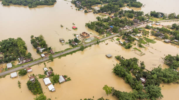
Flow Models in Hydrology
Hydrological flow models are built on the concept of the return period. Two equivalent defini-tions have become established, of which one — cited here, relating to the so-called uncondi-tional return period — is used considerably more frequently. The return period indicates the time until the first extreme event — that is, one whose magnitude exceeds a certain fixed threshold. In hydrological models, researchers most often make use of the block maxima method.
In this approach, only a single flow value is drawn from a given period (block) — most often a single year — namely, the maximum value; and this value, together with other such values drawn from other blocks, is subjected to statistical modeling. Adopting such an ap-proach gives rise, in a natural manner, to the concept of the T-period flood — for example, the 100-year flood, that is, a flood occurring once every T (every 100) blocks, and thus once every 100 years. This is precisely the return period.
The Assumption of Stationarity and Independence
It is self-evident within hydrology that the methods described above for determining the return period, as well as the number of events over the period T, can be applied only if two fundamental conditions are satisfied: (i) extreme events are drawn from a stationary distribution; and (ii) they are independent of one another. Both, when satisfied, are equivalent to ensuring the i.i.d. condition (independent and identically distributed) for the distribution of the phenomenon, and to ensuring the constancy of the exceedance probability p — the probability of exceeding a certain water level. Within hydrology, this is to be understood as meaning that, over the period observed (e.g., T = 100 years), we assume constant conditions — that is, an unchanging distribution and its variance (an unchanging probability p) — as well as the independence of successive observations drawn from such a flow distribution. Assumptions of this kind were formulated at the time when the scope of methods and approaches for modeling the flood phenomenon was being established. Doubts as to the validity of adopting such conditions, which were already emerging at that time within the research community, were commented on by Gumbel in 1941 in the following manner (Volpi et al., 2015):
In order to apply any theory, we have to suppose that the data are homogeneous, i.e., that no systematical change of climate and no important change in the basin have occurred within the observation period and that no such changes will take place in the period for which extrapolations are made. It is only under these obvious conditions that forecasts can be made.
(Volpi et al., 2015)
The hydrological models that have been in operation over the past hundred years in the United States, as well as the models widely applied in other countries, have thus been based on i.i.d. assumptions. This was an assumption that was necessary, and one not subject to discussion.
Parametrizations of the Return Period in the World of Physical Phenomena
Within the domain of physical phenomena, researchers and the institutions engaged in describing them have developed various calibrations of the return period, each useful in the processes for which they are applied. For instance, for modeling phenomena such as earthquakes, a calibration at the level of a 2,475-year event has been adopted; for extreme events whose materialization might occur on the site of a nuclear power plant, this figure is 409 years; while for flood infrastructure, we speak of a 100-year event.
Table 1: Expected Return Period (T-Years) for Various Physical Phenomena
| Field | Expected Return Period (T-Years) | Source |
|---|---|---|
| Earthquakes | 2475 | NEHRP (2010) |
| Retirement portfolios | 585 | Ameriks et al. (2001) and Stout and Mitchell (2006) |
| Nuclear power plants | 409 | United States National Nuclear Regulatory Commission (1975) |
| Flood insurance | 105 | FEMA |
| Flood infrastructure | 100 | Yen (1970) |
Source: Based on Read and Vogel (2015)
Notes: It should be added that, in models of physical phenomena, researchers also make use of a further parameter — the planning horizon — which has been omitted here.
The End of the Stationarity Assumption
At the outset of the twenty-first century, Milly et al. (2008), in a widely noted article titled "Stationarity Is Dead: Whither Water Management," concluded: "Systems for management of water throughout the developed world have been designed and operated under the assumption of stationarity." At the time, in 2008, they valued the global investment in water infrastructure, designed on the basis of models employing the stationarity condition, at US$500 billion. They described the concept of stationarity, as employed in hydrology over the preceding several decades of the twentieth century, as: "the idea that natural systems fluctuate within an unchanging envelope of variability."
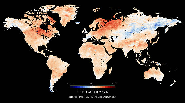
Milly et al. go on to state that this envelope of natural variability has been exceeded, and formulate their central thesis: stationarity is dead. Pointing to climate change as the principal cause of the breach of this hitherto inviolable condition, they write emphatically: "we assert that stationarity is dead and should no longer serve as a central, default assumption in water-resource risk assessment and planning." Drawing on projections of the average level of global surface water runoff for the year 2050, and comparing these levels to observations from the period 1900–1970, they point to a substantial change — one that cannot be captured within a variance understood in stationary terms. In addition, addressing the relationship between changes at the level of the mean and those at the level of distant quantiles, they argue that "paleohydrologic studies suggest that small changes in mean climate might produce large changes in extremes […]," and, with respect to the resilience of currently constructed safety systems, that "projected changes in runoff during the multidecade lifetime of major water infrastructure projects begun now are large enough to push hydroclimate beyond the range of historical behaviors." At the end, the authors propose adapting existing models so as to enable them to capture the temporal evolution of the probability distribution, together with an estimate of the associated uncertainty.
The authors' closing statement — "stationarity cannot be revived" — provoked, within the hydrological community, a debate on the mortality and immortality of stationarity. This question became the dominant research problem within twenty-first-century hydrology (e.g., Cooley, 2013; Salas and Obeysekera, 2014; Du et al., 2015; Read and Vogel, 2015).
The Return Period Under Conditions of Non-Stationarity
Read and Vogel (2015) examined the usefulness of the concept of the expected return period under conditions of non-stationarity, while retaining the assumption of temporal independence. They undertook an attempt to describe the flow phenomenon precisely under such non-stationary conditions — that is, with non-stationary return periods. They demonstrated that, under such unstable conditions, the concept of the T-year flood changes over time. For instance, the 100-year flood, 50 years from now, will be 1.6 times larger than today's 100-year flood. There is thus no single value corresponding to the 100-year flood. This may, of course, give rise to further interpretive — and consequently communicative — complications, with respect to a return-period definition that already causes considerable difficulty even under stationary conditions. It may be, however, that a time-varying exceedance probability p (that is, put differently, 1/T) renders this new, non-stationary concept of the return period altogether devoid of usefulness. What is more, the very form of the non-stationarity may itself be variable, which further complicates any modeling approach whatsoever.
The Return Period Under Conditions of Temporal Dependence Among Observations
Volpi et al. (2015), in the reverse of Read and Vogel (2015), relaxed the assumption of temporal independence while retaining the assumption of stationarity. They constructed a time-dependent model, characterized by the presence of properties commonly found in phenomena of this kind: (i) persistence, and (ii) clustering. The first property denotes a tendency for the same state to persist over an extended period; the second, a tendency for extreme events to cluster within neighboring periods. Using a model built on these assumptions, the authors tested the usefulness of the return period definition. They conclude: "[…] in the context of time-dependent processes, the return period might not represent an exhaustive measure of the probability of failure, and that its blind application could lead to misleading results." Above all, however, the authors drew attention to the difference in results depending on the definition of the return period adopted. They note that, whereas under conditions of temporal independence both commonly used definitions (the unconditional return period and the conditional return period) are equivalent, under conditions of temporal dependence, different definitions yield different results. In addition, they demonstrate that readings of the classically understood return period, under conditions of temporal dependence, lead to erroneous interpretations, and they propose an alternative measure — the equivalent return period — which serves as the counterpart of the return period under conditions of temporal dependence.
Criticism of the Probabilistic Approach in Hydrology
In the field of hydrological research, a certain turning point, it would seem, can be observed: growing criticism of traditional statistical methods, and a shift toward mechanistic descriptions of phenomena. Over the past two decades, an increasing number of publications have appeared subjecting to criticism the assumption of the random character of the flow phenomenon, and of the floods that result from it. Merz and Blöschl (2008) cite Klemeš's statement: "If more light is to be shed on the probabilities of hydrological events, then it will have to come from more information on the physics of the phenomena, not from more mathematics." The authors go on to state that the hydrological literature has focused excessively on solving technical estimation problems (distribution fitting, parametrization methods), neglecting the wealth of hydrological knowledge in the process. They propose shifting the center of gravity of research, pointing out that there exists a rich diversity of hydrological processes, often specific to a given location, which cannot be fully captured by formal statistical methods.
Dawdy, Griffis, and Gupta (2012), lending support to this line of argument, question the unrealistic assumption of stationarity — that is, the assumption that the future can be predicted by means of a model of the past. At the same time, they point to the insurmountable limitations of traditional statistical models. Despite the many improvements made to such models over time, they remain, they argue, a black box, closed off from knowledge of the physical processes actually taking place.
Milly et al. (2008) point, it would seem aptly, to a necessary change in the philosophy of modeling. A model, they argue, should not be the central point of reference, but merely an aid in synthesizing observations: "Modeling should be used to synthesize observations; it can never replace them."
A New Perspective on the Description of Physical Phenomena
This emerging trend, moving toward a mechanistic approach to the construction of resilience systems, in a certain sense renders the ongoing probabilistic debates moot. Within such a new paradigm, it is no longer necessary to determine the exceedance probability, nor the associated concept of the return period, nor any of the other concepts deriving from it. The recently observed problem of non-stationarity in physical phenomena, and the question of the independence of random variables, cease to be of consequence. Consequently, all attempts to resolve problems of this type — that is, problems whose very definitions were constructed on the plane of statistics, or, more broadly, of probability theory — may likewise be rendered moot.
As can be seen, within the world of natural phenomena — which the scientific community has studied for over a century, and for the description of which the entire, sophisticated statistical apparatus was developed — the fundamental assumptions underlying the models widely applied in this domain are increasingly being called into question. Stationarity and the independence of random variables — axioms indispensable to this statistical architecture — have vanished.
KEY TAKEAWAYS
What is more, the entire probabilistic edifice — the founding idea for problems of this class — is beginning to be widely challenged. Perhaps statistics and its tools are not, after all, the best instrument for describing phenomena of such importance to society. Such is the current state of the debate within this domain of phenomena — one relatively amenable to statistical description: natural phenomena, relatively stable and well understood.
What, then, can be said of the possibility of statistically modeling phenomena that are far less well understood, yet far more dynamic — phenomena that play themselves out on a social substrate, marked by the generic unpredictability of human behavior, in an era of exponentially accelerating civilizational change? ■

Maciej Buczak
Risk management professional with 8+ years validating financial models in banking, currently teaching risk management and econometrics in Warsaw. His research questions the paradigmatic foundations of financial risk architecture — from VaR to AMA and IRB — drawing on extreme value theory.
References Academic sources cited throughout this article — click to expand the full list
Balkema, A.A., de Haan, L. (1974), Residual Life Time at Great Age, The Annals of Probability, Vol. 2, No. 5, pp. 792-804.
Cooley, D. (2013), Return periods and return levels under climate change, in: A. AghaKouchak, D. Easterling, K. Hsu, S. Schubert, S. Sorooshian (eds.), Extremes in a Changing Climate: Detection, Analysis, and Uncertainty, pp. 97-114, Springer, New York.
Dawdy, D.R., Griffis, V.W., Gupta, V.K. (2012), Regional flood-frequency analysis: How we got here and where we are going, Journal of Hydrologic Engineering, 17(9), pp. 953-959.
De Haan, L. (1990), Fighting the arch-enemy with mathematics, Statistica Neerlandica, Vol. 44, No. 2, pp. 45-68.
Du, T., Xiong, L., Xu, C.-Y., Gippel, C., Guo, S., Liu, P. (2015), Return period and risk analysis of nonstationary low-flow series under climate change, Journal of Hydrology, 527, pp. 220-227.
Fisher, R.A., Tippett, L.H.C. (1928), Limiting forms of the frequency distribution of the largest or smallest member of a sample, Mathematical Proceedings of the Cambridge Philosophical Society, Vol. 24, No. 2, pp. 180-190.
Foster, H.A. (1924), Theoretical Frequency Curves and Their Application to Engineering Problems, Transactions of the American Society of Civil Engineers, Vol. 87, No. 1, pp. 142-173.
Fuller, W.E. (1914), Flood flows, Transactions of the American Society of Civil Engineers, Vol. 77, No. 1, pp. 564-617.
Hazen, A. (1914), Discussion on "Flood flows" by W.E. Fuller, Transactions of the American Society of Civil Engineers, Vol. 77, pp. 626-632.
Merz, R., Blöschl, G. (2008), Flood frequency hydrology: 1. Temporal, spatial, and causal expansion of information, Water Resources Research, 44, W08432.
Milly, P.C.D., Betancourt, J., Falkenmark, M., Hirsch, R.M., Kundzewicz, Z.W., Lettenmair, D.P., Stouffer, R.J. (2008), Stationarity is dead: Whither water management, Science, 319, pp. 573-574.
Pickands, J. (1975), Statistical Inference Using Extreme Order Statistics, The Annals of Statistics, Vol. 3, No. 1, pp. 119-131.
Read, L.K., Vogel, R.M. (2015), Reliability, return periods, and risk under nonstationarity, Water Resources Research, Vol. 51, No. 8, pp. 6381-6398.
Salas, J.D., Obeysekera, J. (2014), Revisiting the concepts of return period and risk for nonstationary hydrologic extreme events, Journal of Hydrologic Engineering, 19(3), pp. 554-568.
Volpi, E., Fiori, A., Grimaldi, S., Lombardo, F., Koutsoyiannis, D. (2015), One hundred years of return period: Strengths and limitations, Water Resources Research, Vol. 51, No. 10, pp. 8570-8585.
Vogel, R., Wilson, I. (1996), The probability distribution of annual maximum, minimum and average streamflow in the United States, Journal of Hydrologic Engineering, 1, pp. 69-76.


Reader Discussion
Share
your thoughts
Tip: Choose the category that best describes your comment. This may help other readers. See more