
Share this article
I Can't Predict a 1,000-Year Catastrophe
H ow many years must one wait to experience the financial catastrophe against which today's regulatory system protects us? The answer, which can be found in supervisory documents, is: a thousand years. The 0.999 quantile — the central parameter of the Basel safety system — is there explicitly interpreted as an event occurring once every thousand years. This formulation, reproduced without further comment in academic textbooks and in sectoral practice, is the point of departure for the present paper.
CREDIT.risk
OPERATIONAL.risk
MARKET.risk
MODEL.risk
SYSTEMIC.risk
The criticism of the Value at Risk concept, along with the statistical apparatus accompanying it, already has a rich tradition. Artzner et al. (1999), Danielsson (2000), Danielsson et al. (2001), among others, have repeatedly pointed out that the estimation of distant distribution quantiles — such as 0.99 or 0.999 — is a task lying at the very limit of what available statistical methods can accomplish, one burdened by errors reaching entire orders of magnitude. This problem, well recognized and repeatedly described in the literature, is not the subject of the present paper. This article poses a different, narrower question — one that, it would seem, has not thus far been addressed directly: not whether we are able to reliably estimate the value located at the 0.999 quantile, but rather how the interpretation of the 0.999 quantile as an event occurring "once in 1,000 years" is to be understood. In other words, the object of the analysis is not the quality of estimation at the distant quantiles of distributions, but the validity of the temporal interpretation itself that is ascribed to the results of such estimation.
This distinction is key to understanding the contribution of this paper. Even if one had at one's disposal an ideal risk model, free of estimation error, the question of what the claim that its result corresponds to a 1,000-year event actually means would remain open. The temporal interpretation of the quantile is not, as this article seeks to demonstrate, a necessary element, nor one that follows intrinsically from the construction of such a model. It is a convention — borrowed, though never explicitly identified as such, from an entirely different field: hydrology, where, at the turn of the nineteenth and twentieth centuries, the concept of the return period was developed to describe phenomena such as the hundred-year flood. This convention, however, requires an additional assumption — the indexing of successive realizations of the phenomenon, of successive random variables, by means of time — the validity of which, in the world of socio-economic phenomena, is considerably more difficult to justify than in the world of physical phenomena, governed by fixed astronomical cycles. What is more, hydrology itself, faced with years of criticism (Pielke, 1999; Read and Vogel, 2015; Stedinger, Vogel and Foufoula-Georgiou, 1993), has already revised the way in which this concept is communicated, pointing to its misleading nature. The world of finance, it would seem, has not yet undertaken this reflection.
Download full version of article
Download
01
Problems with the Practical Application of Financial Safety Requirements
The first project of the financial safety architecture was Basel I (1988) — covering credit risk, with capital requirements determined arithmetically. In 1996, an amendment was introduced, incorporating market risk into the concept. The measurement of this risk was entrusted to the VaR concept — a new idea for measuring risk. In 2004, the Basel II package was announced, introducing the concept of internal models and providing corresponding frameworks for credit, operational, and market risk. The final product of the Basel architecture was meant to be an anti-crisis barrier, one that all entities, by means of internal models, were to build together.
The foundation of risk models, across all risk domains, was the VaR method, introduced by J.P. Morgan and Reuters in 1996. The safety level was, in turn, defined, in the language of this very concept, as the distribution quantile at which the VaR reading was to be taken. These quantiles were the extreme levels of 0.999 — for credit and operational risk — and 0.99 — for market risk.
The Problem of Model Verification at a Distant Quantile
A common problem afflicting models built on this conceptual matrix was the difficulty in verifying their correctness. There exist, in essence, no reliable methods for backtesting values at such quantiles. What remains — always useful — is an assessment of the model's consistency with reality. The process of verifying a model's results at the 0.999 quantile might proceed as follows
What are we meant to be protected against? → Against an extreme event → How extreme? → At the 0.999 quantile → What does that mean? What does it look like on the map of reality, on the map of real threats?
The last question is not easy to answer. Is the capital determined by the model at the 0.999 quantile, say, USD 100 million, sufficient to cover a real, extreme situation that threatens us? Perhaps the best way to connect the model with reality is to construct such an extreme scenario as actually threatens us. If our capital exceeds the material scale of the materialization of such an imagined, but real, scenario — we are safe. If not — the capital is too low. In attempting to construct such an extreme scenario, however, we again encounter the same barrier:
→ How is the extremity of the scenario to be formulated? → At the level of the 0.999 quantile → But what does an extreme situation at the 0.999 level look like? What does the 99.9% quantile mean?
Anyone who has taken part in, or at least moderated, various scenario analyses — for example, within the scenario methods envisaged under the AMA framework in operational risk — understands the problematic nature of questions of this type. Participants in such scenario panels, experts in banking risk, are unable to process, interpret, and apply to reality a parameter such as the 0.999 quantile. To ensure credible results from the scenario process, an interpretation of such a numerically expressed quantile is needed. A hint can be found in supervisory regulations. To the question of how the 0.999 quantile is to be understood, the regulator answers:
→ The 0.999 quantile is an event occurring once every 1,000 years.
What now?
→ Let us imagine such a 1,000-year event, and consider what shape and course it would take, and what material scale it might assume → Let us now compare this imagined event with the capital buffer determined by the model (at the 0.999 quantile), which is meant to protect us against such an event → If the capital covers the material scale of the 1,000-year event — we are safe.
Unfortunately, this thought process cannot be carried out. We become stuck at the point "let us imagine a 1,000-year event." An attempt to imagine a 1,000-year event forward, 1,000 years from now, is entirely devoid of sense. A seemingly helpful attempt to imagine a 1,000-year event backward, on the pages of history, likewise proves useless. Neither the reality 1,000 years hence nor the reality 1,000 years past bears any resemblance whatsoever to the world in which the model operates and to which it is meant to relate.
The quantile calibration levels formulated within the financial safety architecture are, in essence, the central parameters of this system. It is these that determine the level of extremity, and thus the levels of capital that are meant to govern this safety. For credit risk, the safety level was encoded within the IRB calculation formula - Art. 154 (EU, CRR, 2013):
$$
RW = \left\{ LGD \cdot N\left( \frac{1}{\sqrt{1-R}} \cdot G(PD) + \sqrt{\frac{R}{1-R}} \cdot G(0{,}999) \right) - LGD \cdot PD \right\} \cdot 12{,}5 \cdot 1{,}06
$$
where G(0.999) is the quantile of the systematic factor at the 0.999 level, and N(...) is the conditional probability of default under the worst-case macroeconomic scenario, read off the normal distribution.
02
The Central Parameter of the Safety Architecture — the 0.999 Quantile
The 0.999 quantile relates directly to the systematic factor M in the ASRF model, corresponding to a 99.9% confidence level, which can be written as (Jorion, 2007): "P(− M ≤ m) = 0.999, or M = N⁻¹(0.999)." The value of the 99.9% quantile in the IRB model is thus a level of extremity established within the calculation formula itself, for systematic risk shared by all market participants. In the domain of operational risk, for the internal model (AMA), the safety level and the time horizon were formulated in the document (EU, CRR, 2013), Article 322(2)(a): "The operational risk measure shall capture potentially severe tail events, achieving a soundness standard comparable to a 99.9% confidence interval over a one year period." The supervisor borrowed this calibration level from credit risk: "[…] soundness standard comparable to that of the internal ratings-based approach for credit risk, (i.e. comparable to a one year holding period and a 99.9th percentile confidence interval)."
For both risks — credit and operational — an annual time horizon was set. For market risk, which is addressed to a lesser extent in this paper (there is no talk here of a 1,000-year event), the safety level was set at the 0.99 quantile, at a 10-day time horizon. Temporal interpretations were not included in the principal supervisory documents.
03
The Temporal Interpretation of Distant Quantiles — 0.999 as Once in 1,000 Years
The temporal interpretation, with respect to the IRB model, appears in a lower-order document, the guidelines (BIS, BCBS, 2005):
The confidence level is fixed at 99.9%, i.e. an institution is expected to suffer losses that exceed its level of tier 1 and tier 2 capital on average once in a thousand years. […] The confidence level is included into the Basel risk weight formulas […]
(BIS, BCBS, 2005)
The supervisor explains that the 0.999 quantile in the credit risk model has been embedded directly within the formula used to determine risk weights. What matters most, however, in the context of the argument developed here, is that the document explicitly indicates an interpretation of the reading of the 0.999 quantile as once in 1,000 years. It does not, however, offer any justification for this whatsoever.
The temporal interpretation of the 0.999 quantile for operational risk models (AMA) appears in a lower-order document, the guidelines (BIS, BCBS, 2011): "Just in limited cases, for example when the biggest data point is demonstrated to be larger or equal in amount to the event that occurs less than once in 1000 years […]"
In operational risk, then, following the interpretation developed in the domain of credit risk, the same manner of defining extremity was adopted — as an event occurring no more frequently than once in 1,000 years. Importantly, here too no reasoning is presented for such an approach, and this interpretation of the quantile is not justified.
As can be seen, the regulator has explicitly indicated how the values at the 0.999 quantile are to be read — as once-in-1,000-year events. This, however, does not resolve the problem of model verification derived earlier. For how is one to imagine a 1,000-year event? It may be worth verifying the correctness of such an interpretation within the academic literature.
The Widespread Interpretation of the 0.999 Quantile as Once in 1,000 Years
When we turn to the academic literature, it becomes apparent that the interpretation of distant quantiles as 1,000-year events is widespread. Jorion (2007) essentially repeats the regulator's formula:
[…] to cover unexpected losses over a 1-year horizon at the 99.9 percent confidence level. This seems very conservative. It means that a bank would fail, on average, once in a thousand years.
Jorion (2007)
Hull (2018) does the same: the capital "should be sufficient to cover unexpected losses of a magnitude that, over the coming year, should not, with 99.9% probability, be exceeded. WCDR denotes the probability of default at a level that (theoretically) occurs once every thousand years." Genest and Brie (2013): "That's why the confidence level is set at 99.9%. It means a bank can have losses that exceed its tier 1 and tier 2 capital on average once in a thousand years." Milonas and van Vuuren (2024): "[…] a confidence level of 99.9% is sufficient since losses that exceed the ULs are predicted to occur only every 1000 years because the PDs used are annual PDs." Similar temporal interpretations — likewise applied to other quantile levels — can be found in the works of Danielsson (2000), Reinhart and Rogoff (2009), Laubsch and Ulmer (1999), and Kiema and Jokivuolle (2013).
The temporal interpretation of quantiles is thus widespread. Interestingly, it is difficult to find any derivation for precisely this temporal understanding of such extreme quantiles.
Let us return, however, to the problem of verifying the model's consistency — its 0.999 quantile — against reality:
→ Let us imagine such a 1,000-year event, and consider what shape and course it would take, and what material scale it might assume → Let us now compare this imagined event with the capital buffer determined by the model (at the 0.999 quantile), which is meant to protect us against such an event → If the capital covers the material scale of the 1,000-year event — we are safe.
How, then, is one to imagine a 1,000-year event? It was decided to seek the answer more broadly, in other domains, where similar definitions might operate.
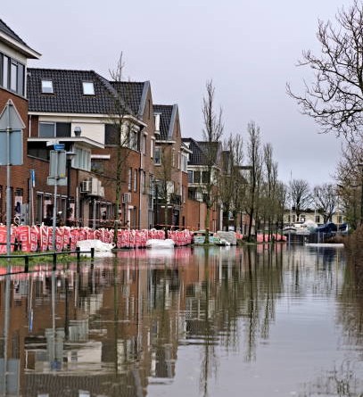
This problem is best analyzed using the example of hydrology, where the concept of the hundred-year flood has a long tradition. A good point of reference is the well-known Dyke Project — the flood-defense dike project constructed following the 1953 flood. The height of the dikes was determined precisely on the basis of statistical methods, drawing on historical data, including the 1570 flood observation. Ultimately, by means of appropriate functions, the concept of a 10,000-year event was formulated, which became the basis for the flood safety system. How, though, can a 1,000- or 10,000-year event be derived?
Such a derivation can be carried out on the basis of the concept of the return period. It was first formulated by Fuller in 1914. Later, Hazen (1914) placed this concept on the probability map, and, subsequently, through the work of Foster (1924) and Gumbel (1941), as well as the ideas underlying extreme value modeling (EVT I), this definition came to be widely adopted. The most important institutes engaged in modeling water flows make use of precisely this concept, along with the corresponding probability distributions.
04
The World of Nature — Modeling Catastrophes
Return Period and T-Period Event
Fuller derived the definition of the return period as follows:
$$
Q_T = CA^{0.8}\left[1 + 0.8\log_{10}(T)\right]\left(1 + 2A^{-0.3}\right)
$$
where Q_T is the maximum flow, and T is precisely the return period. Increasing T is equivalent to increasing rarity — thus, for a larger T (a rarer event), a larger flow Q_T (a larger flood) is to be expected. It should be noted that this equation is deterministic in nature — there is, as yet, no assumption here of the randomness of the phenomenon.
Once, however, we describe the phenomenon as random, we have:
$$
P(X > x_p) = 1 - p
$$
that is, the probability of exceeding a certain level x_p — the level of the rare event.
Dyke Project
The Delta Works (also known as the Dyke Project) is a Dutch system of flood-defense structures — dams, sluices, dikes, and storm surge barriers — protecting the southwestern part of the Netherlands from the North Sea. It was built in response to the catastrophic flood of the night of January 31/February 1, 1953, in which 1,836 people died and more than 2,000 km² of land was flooded. Construction lasted from 1954 to 1997. Rather than relying solely on the analysis of past floods, the project's creators developed a novel statistical approach to determining the required dike height — one accounting for extremely rare events, measured in thousands of years.
The return period for such an event is:
$$
T = \frac{1}{1-p}
$$
For an exceedance probability of 1 − p = 0.01, the return period amounts to 100. What remains is the question of the unit for T = 100. It is worth noting that flow researchers made use of the so-called block maxima method (EVT I is likewise built on this method). This means that, from all flow observations, only a single one is selected — the maximum for a given period (block). The period is most often a year. From this, T = 100 years emerges naturally, giving us a 100-year event.
It should be added here that the return period T is the expected return period. In reality, this value is described by a distribution — the binomial distribution, which is the distribution of binary variables (exceedance, no exceedance). For large samples, this may, of course, be approximated by the Poisson or normal distribution.
For a period of T = 100, there is thus a 36% chance of a single exceedance, an 18% chance of 2 exceedances within this period, and so on. There may also be no exceedance at all within the period T = 100 — a 36% chance.
The problem can be presented differently. Using the geometric (or exponential) distribution, one can determine, from this distribution, the moment of first exceedance. If the result is read from the probability function, one obtains the chance of a first exceedance at a specific moment k; if from the cumulative distribution function, the chance of a first exceedance occurring by moment k.
Table 1: Probabilities of k exceedances for a 100-year event (T = 100) and a 1,000-year event (T = 1,000)
| Number of Exceedances |
Period T=100 100-Year Event |
Period T=1000 1,000-Year Event |
|---|---|---|
| k | Poisson (λ = 1) | Poisson (λ = 1) |
| 0 | 0.3679 | 0.3679 |
| 1 | 0.3679 | 0.3679 |
| 2 | 0.1839 | 0.1839 |
| 3 | 0.0613 | 0.0613 |
| 4 | 0.0153 | 0.0153 |
| 5 | 0.0031 | 0.0031 |
Source: own elaboration
In summary, a 100-year event will, on average, occur once within a period of 100 years, and the average waiting time for an event of this kind is 100 years (Table 3). It may nonetheless happen that such a 100-year event does not occur at all within 100 years, or that several such events occur within that period. The first occurrence of a 100-year event may take place after just a single year (a 1.00% chance); within the first 10 years, the chance of such an event occurring is 9.56%; and within 50 years, it is 39.5%. Interestingly, within the 100-year period under study, the first 100-year event has only a 63% chance of appearing. Within 500 years, however, it should appear with a probability of 99%. Analogous reasoning applies in the case of the 1,000-year event observed over a period of 1,000 years.
Table 3: Probability of the first exceedance occurring exactly in year k, and the probability of the first exceedance occurring by year k, for the 100-year event (with period T = 100 years) and the 1,000-year event (with period T = 1,000 years)
| Period T=100 100-Year Event |
Period T=1000 1,000-Year Event |
||||
|---|---|---|---|---|---|
| k (years) | P(K=k) | P(K≤k) | k (years) | P(K=k) | P(K≤k) |
| 1 | 1.00% | 1.00% | 1 | 0.100% | 0.10% |
| 2 | 0.99% | 1.99% | 2 | 0.099% | 0.19% |
| 5 | 0.96% | 4.90% | 5 | 0.099% | 0.49% |
| 10 | 0.91% | 9.56% | 10 | 0.099% | 0.99% |
| 20 | 0.82% | 18.21% | 20 | 0.098% | 1.98% |
| 50 | 0.61% | 39.50% | 50 | 0.095% | 4.87% |
| 69 | 0.50% | ≈50% Median | 100 | 0.090% | 9.51% |
| 100 | 0.37% | 63.40% | 200 | 0.082% | 18.12% |
| 150 | 0.22% | 77.69% | 500 | 0.061% | 39.34% |
| 200 | 0.14% | 86.58% | 693 | 0.050% | 50% Median |
| 300 | 0.05% | 95.02% | 1000 | 0.037% | 63.21% |
| 500 | 0.01% | 99.34% | 2000 | 0.013% | 86.46% |
| 5000 | 0.001% | 99.32% | |||
| 10000 | 0.000% | 99.99% | |||
Source: own elaboration
05
The World of Risk and Its Definitions of Rare Events
The Value at Risk method, developed by J.P. Morgan/Reuters (1996), draws on this same conceptual system as the one indicated above. The basic object is the threshold of the extreme event — VaR itself — and the central definition is the probability of exceeding this VaR level:
Value-at-Risk is a measure of the maximum potential change in value of a portfolio of financial instruments with a given probability over a pre-set horizon. VaR answers the question: how much can I lose with x% probability over a given time horizon.
J.P.Morgan/Reuters (1996),
We thus have:
$$
P(X > VaR) = 1 - p
$$
The key parameter here is the predefined extremity level, the quantile p. If we take p to be, say, 0.999, then the exceedance probability is 1 − p = 0.001. The level p is also referred to as the confidence level.
It is precisely on this concept — Value at Risk — that the financial safety architecture has been built. Credit, operational, and market risk models, as well as various modeling constructs within the domain of internal capital, derive their final readings precisely by means of the VaR method. The key parameter is the extremity level p, predefined at the following levels: 0.999 for credit and operational risk, 0.99 for market risk.
From the VaR formula, the definition of the return period can likewise be derived. Let us assume that a model describes a bank's risk profile, the variable R. This risk may materialize with the probabilities embedded within the very definition of this variable. For instance, with probability \(p = 0.001\), an extreme value — the VaR level — may materialize. An exceedance of the VaR level may thus occur. We may also consider a sequence of different risk profiles \((R_i)\). This can likewise be written as a sequence of binary variables \(\left(I_{\{R_i > VaR\}}\right)\). This, in turn, can take on only two values:
$$
I_{\{R_i>VaR\}} = \begin{cases} 1, & \text{if } R_i > VaR \text{ (a VaR exceedance)} \text{ — "success"} \\ 0, & \text{if } R_i \le VaR \text{ (no exceedance)} \text{ — "failure"} \end{cases}
$$
One can ask the question: which of the risk profiles R belonging to the index set I will assume a value higher than the VaR level. This can be written as:
$$
L(VaR) = \min\{i \ge 1 : R_i > VaR\}
$$
which will denote the index of the risk profile at which an exceedance of the VaR level — that is, for instance, an exceedance of the 0.999 quantile — occurs for the first time. Now, if we adopt the assumption that the index in this sequence is time, and that the horizon is annual, then, for p = 0.999, we have an exceedance chance of 0.001, meaning an exceedance occurring once every 1,000 occurrences — that is, once every 1,000 annual periods. The concept of the 1,000-year event thus emerges.
Statistical Properties versus the Question of Time
A distinction needs to be drawn between the statistical properties from which probability readings derive, and the temporal interpretation, which does not follow from these properties, but arises in a different — "non-statistical" — manner. A reading of the exceedance probability, say 0.001, derives from the binomial or geometric distribution — depending on what one wishes to read off. These distributions, in turn, are formed from the aggregate phenomenon of many binary variables (exceedance, no exceedance). These binary variables simply compose into such distributions. What remains is the question of indexing these binary variables. This can be done in various ways, and the appropriate definition of the return period emerges depending on the method chosen. If we assign no interpretation at all, we speak of a "1,000-index" event — the expected value of the exceedance occurs at the 1,000th binary variable (marked with index i = 1,000). If we use the index to denote different institutions and their risk profiles, we obtain an event occurring once every 1,000 institutions; if, instead, we build 1,000 different models for a risk profile, the exceedance occurs at the 1,000th model. As can be seen, indexing by time is merely a convention, and it is only under this convention that a 1,000-year event can arise. What matters here is that the emergence of the 1,000-year event does not follow from the statistical properties, but precisely from the indexing convention.
Indexing by Time - Tacit Assumption
Embrechts, Klüppelberg, and Mikosch (1997), in deriving an example illustrating the concept of the return period, write: "Here we tacitly assumed that a structure failure for each year i can be modeled through the event \(\{X_i > u\}\)." We thus see the operation of a "tacit assumption" of indexing by time. In hydrology, this assumption is justified. The block maxima method adopted there imposes annual periods — annual maximum flows are modeled. This is consistent with the astronomical cycles of nature — the Earth's orbital motion. In the case of socio-economic phenomena, this is no longer so self-evident. It is difficult to say how long individual phenomena last — those that underlie the binary variables which, taken together, form the binomial (or geometric) distribution. In order to compose such a distribution, however, the independence of these variables is required. They must play themselves out, must exhaust their probabilities (much as a game of poker must be played through to its end — and each game, together with its associated probabilities, may take a different amount of time). If they are not played through to completion, the probabilities will bleed into one another across these variables, and they will not, in that case, be independent. It is then impossible to compose a binomial distribution. Nor is it possible, in that case, to obtain a reliable quantile reading from such a distribution — there is, accordingly, no 1,000-year event. How long do socio-economic phenomena last, and is this duration constant? It is not known. This is difficult to calculate. It is also doubtful that it would always be the same duration. The world, after all, is accelerating, and phenomena that once took many years to unfold may now play themselves out over a matter of months.
Notwithstanding this, the world of economics applies precisely this "tacit assumption" of indexing by time, deriving from it concepts such as the 1,000-year event.
Once in 1,000 Years Lies Outside the Model
Having traced the reasoning presented above, it must be concluded that the definition of the 1,000-year event is not built into the risk model. The model returns loss values, and these can only be interpreted on the map of probability. The 0.999 quantile of such a model (risk profile) tells us only the loss value standing at that quantile, and the chance of such a loss (or a greater one) occurring. The probabilities read off from this distribution pertain to a "single draw" from the variable R — or, put differently, to a single loss-generating process arising from the variable R. This means that we are speaking of the chance of exceeding the loss value located at the 0.999 quantile here and now — that is, within the period defined by the time horizon (e.g., a year). This is the only interpretation of readings from the random variable to which we are entitled.
06
In the World of Risk Models, the 1,000-Year Event Is an Empty Artifact
The concept of the 1,000-year event arises outside the model (or the risk profile) — only once we carry out the mechanics of composing risk profiles into a sequence, and index that sequence by time, under the "tacit assumption."
If, then, the concept of the T-period event is not written into the mechanics of the model — if it is an external object — what purpose is served by a definition formulated in this way, and by the underlying process of sequencing the variables on which it rests? What is its practical application?
Backtesting — The Natural Domain for the T-Period Event
The application of the mechanics described above became sanctioned within the world of finance in the context of the problem of verifying extreme value models. Reasoning of this kind was already presented in the J.P. Morgan (1996) study, as well as in the work of Kupiec (1995). Testing exceedances precisely by arranging independent binary variables into a sequence, along the time axis, relates directly to these mechanics. The supervisor sanctioned such a backtesting method for market risk. There, exceedances of the 0.99 quantile of risk models, observable in days, are tested. This gives rise to the concept of a T-day event — for instance, a 100-day event. A problem of stationarity naturally arises here, though for periods measured in days this would seem to be a solvable one. For credit and operational risk — where, on account of the higher level of difficulty (the 0.999 quantile at an annual horizon), a verification tool of this kind would be of even greater usefulness — the supervisor formulated no backtesting methods. This is, of course, understandable. For how, indeed, is one to test a 1,000-year event? Institutions building such models were nonetheless left without recourse. No tools exist for verifying these super-extreme models. Jorion (2007) commented on this, anticipating, as it were, the course of events to come, writing: "The true test of these new models will come during a major economic downturn."
With respect to the concept of the 1,000-year event, it must be noted here that, owing to the absence of a natural domain within which such an event could be derived — the domain of the backtesting procedure (where the concept of the 100-day event was, precisely, derived) — this definition vanishes. There is no way to derive a 1,000-year event.
Model Calibration Invalidates the "Once in 1,000 Years" Definition
What, however, if we did have such a test at our disposal — for instance, by shifting the tested quantile to the 0.9 level, which would make it feasible, in that case, to test a 10-year event? We would then still need to ensure stationarity over such a ten-year period. This, however, may prove difficult. Perhaps, though, this is not a problem at all. Let us note that models are calibrated on a continuous basis. This, in turn, anchors the model in current reality. The model, through calibration, shifts along with a changing reality. Each time, after every such shift, it indicates the probability of a VaR exceedance here and now, over the coming year. The requirement of calibration thus removes, from the conceptual space, any notion of a T-period event whatsoever. What concerns us is current reality, to which we adapt on a continuous basis.
Let us note that matters stand differently in the world of hydrology. Flood barriers cannot be recalibrated every year; they cannot be raised and lowered on such cycles — this would be too costly. Such barriers must, therefore, be resilient over a certain time horizon. There, then, the concept of a T-period event — say, the 100-year flood — is considerably more natural.
Once in 1,000 Years — An Empty Artifact
As has been attempted to demonstrate here, the 1,000-year event is not a definition built into a bank's risk profile, and is thus not a concept that can be read off from the mechanics of a risk model. This concept is merely a certain statistical label, a shorthand, an approximation, which, one must presume, was intended to help in describing extreme events. It must be borne in mind, however, that this label was derived on a certain conceptual map, and retains its meaning only within that map. In the world of finance, the natural domain in which such a conceptual map is employed — and along with it, the concept of the T-period event sanctioned — is the domain of model backtesting. Yet while such a testing procedure was formulated for market risk, it was not formulated for credit and operational risk, where the 0.999 quantile and an annual horizon are at issue. It is thus impossible to derive the concept of the 1,000-year event, for there exists no space within which such a derivation could take place. An attempt to construct such a testing framework, purely theoretical in nature, would encounter a barrier in the form of the absence of stationarity for the phenomenon over such a span of time — which would likewise preclude formulating the concept of the 1,000-year event. Viewed from another angle, the very idea of calibrating models — that is, of adapting them to a changing world — anchors the model in the reality of here and now, and points to a purely probabilistic, rather than temporal, interpretation of the safety levels expressed by the 0.999 quantile. This, too, rules out the possibility of applying an interpretation of the "once in 1,000 years" type.
It would thus seem that the concept of the "once in 1,000 years" event, so widespread in the world of finance, is merely a certain artifact, and, moreover, an empty one. This concept appears to have no explicable application whatsoever. Nor does it add any value — it does not help us better interpret model results against the map of reality as it actually operates, and as it manifests itself in the form of losses recorded on accounting ledgers. Perhaps, then, this concept is simply unnecessary?
Much suggests, then, that we are dealing with an axiomatic vacuum surrounding the definition of the 1,000-year event. This is not, of course, a matter of the broadly understood axiomatic field. On an extensive map of concepts and definitions, the 1,000-year event can indeed be derived — as it was, for instance, within the Dyke Project, in the construction of flood-defense dikes. What is at issue here, rather, is the regulatory space of axioms, practical definitions, and applied approaches. On this particular map, it is difficult to find any sound derivation of the concept of the 1,000-year event as a point of reference for the safety level to which risk models ought to be calibrated.
It would thus seem that the concept of the "once in 1,000 years" event, so widespread in the world of finance, is merely a certain artifact [1] , and, moreover, an empty one. This concept appears to have no explicable application whatsoever. Nor does it add any value — it does not help us better interpret model results against the map of reality as it actually operates, and as it manifests itself in the form of losses recorded on accounting ledgers. Perhaps, then, this concept is simply unnecessary?
07
Problems with False Simplifications
Hydrology Demonstrates the Inapplicability of the 100-Year Flood Definition
The concept of the 100-year flood has recently been going through a difficult period. Pielke (1999) points to a widespread misunderstanding of the flood-frequency concept — that is, of the interpretation of the 100-year flood as an event that may occur once every 100 years: "The 'base flood' is more commonly known as 'the 100-year flood' and is 'probably the most misunderstood floodplain management term.'" And further: "Misconceptions about the meaning of the term creates obstacles to proper understanding of the flood problem and, consequently, the development of effective responses."
Pielke likewise emphasized the practical significance of the misunderstandings that arise from such erroneous definitions:
First, there is general confusion among users of the term about what it means. Some use the term to refer to a flood that occurs every 100 years, as did the Midwestern mayor who stated that ‘after the 1965 flood, they told us this wouldn’t happen again for another 100 years’ (IFMRC, 1994, p. 59). Public confusion is widespread: A farmer suffering through Midwest flooding for the second time in three years complained that ‘Two years ago was supposed to be a 100-year flood, and they’re saying this is a 75-year flood, What kind of sense does that make? You’d think they’d get it right’ (Peterson, 1995).
Pielke (1999),
Read and Vogel (2015), meanwhile, address the social consequences of the misunderstanding of risk:
The consequences of misinterpreting the expected waiting time to an extreme event do not only impact the physical system but also impact perceptions of individuals interacting with the floodplain. […] floodplain residents generally expect to be protected for a particular average return period and have little understanding of the true risk of flooding during their lifetimes.
Read and Vogel (2015)
Read and Vogel conclude that the definition of the return period, and the communication of risk by means of it, is problematic even under conditions of stationarity. This definition does not communicate the true risk of catastrophe. In addition, stakeholders — including policymakers, engineers, insurers, and ordinary citizens — misinterpret the return period precisely as "once in 100 years." Under conditions of non-stationarity [2] , they argue, matters are worse still. The return period no longer depends on a fixed probability p; p now varies over time, which entails an instability in the interpretation of the so-called 100-year flood.
Pielke (1999) states that the only correct definition for the 100-year event is: "[…] flood that has a one percent chance of being exceeded in any given year." He goes on to point out that the 100-year flood is not a natural concept, arising from properties inherent in nature. It is, rather, a definition constructed by scientists and engineers, developed on the basis of historical observations — one that ought to be dynamic, given changing natural conditions and the emergence of new observations. Pielke advocates a return to a legitimate, probability-based communication of risk (a 0.01 chance of exceedance). He notes, however, that supervisory definitions are not easy to change.
The World of Finance Uses an Artifact: The 1,000-Year Event
In the world of finance, where, as has been demonstrated, the concept of the 1,000-year event, sanctioned by the Basel regulations, is widely applied, no debate analogous to the one that took place in hydrology has been carried out. Meanwhile, just as in hydrology, where the 100-year event was at issue, the concept of the 1,000-year event in the world of finance is not a natural concept, arising from inherent laws of nature — in this case, the nature of socio-economic phenomena. It is an engineering construct — in this instance, one belonging to the broadly understood domain of "financial engineering." This construct, however, does not appear to be of any help whatsoever. It offers no assistance in the process of building a model, nor in the process of its empirical verification — no backtesting procedure exists for the 1,000-year event. Nor is it of any use in the qualitative assessment of a model, at the moment when one attempts to confront the model's result at the 0.999 quantile with reality. At that point, the imagined object — the 1,000-year event — likewise offers no guidance whatsoever. This definition is thus useless.

Meanwhile, crises materializing every few years, or perhaps every dozen or so years (see Acharya, Brunnermeier, and Pierret, 2024; and Reinhart and Rogoff, 2009) demonstrate the inadequacy of such a definition. These events ought to prompt deeper reflection on the mechanisms underlying the parametrization of the financial safety system. The concept of the 1,000-year event, or of 1,000-year safety, appears to function, within this system, as a heuristic of false comfort. [3] That this comfort is indeed false is demonstrated precisely each time a crisis materializes. As Pielke (1999) stated, with respect to the world of hydrology, supervisory definitions are not, however, easy to change. This principle, as could be observed over the course of the past twenty years, replicates itself almost verbatim within the world of financial regulation.
The Regulator Introduces an Alternative Line of Reasoning
Interestingly, the regulator also set out a second line of reasoning regarding the 0.999 quantile — one competing with the temporal interpretation (the once-in-1,000-years event). In the document (BIS, BCBS, 2005), it justified the extremity level of the quantile by the need to capture, precisely at that point (at a quantile of the appropriate extremity level), estimation errors, as well as other model uncertainties:
The confidence level is fixed at 99.9% […] This confidence level might seem rather high. […] The high confidence level was also chosen to protect against estimation errors, that might inevitably occur from banks’ internal […] estimation, as well as other model uncertainties.
(BIS, BCBS, 2005)
08
What the Safety System Looks Like in an Unclear Conceptual Environment
It has now become still more difficult to correctly define the meaning of the 0.999 quantile. The supervisor, in adjacent sentences, invokes two different logics. First, it employs a temporal definition, derived, one may presume, from the conceptual system in which the concept of the return period is situated. Immediately thereafter, it states that this extremity level does not stem from an imagined 1,000-year event, but rather from uncertainties originating in the estimation processes. It is difficult to say, then, whether the 0.999 quantile is more a picture of a rarely occurring external event — once every 1,000 years — or a technical safeguard against estimation processes.
Banks Develop Their Own Definitions → Dispersion of Model Results
Ultimately, faced with difficulties in adopting an adequate definition of the 0.999 quantile, each bank, one may presume, develops its own individual definitions. This results in a manner of feeding data into the model that corresponds to the definition adopted for its own purposes — data suited to estimating the value at a quantile understood in this particular, bank-specific way. This, in turn, may lead to discrepancies in capital estimates, potentially reaching entire orders of magnitude, even among very similar banks. Since no clear definition exists, each bank can, after all, conduct its own investigation into the interpretation of the 1,000-year event concept, in its own particular manner.
It is worth recalling, at this point, that the construction of the anti-crisis barrier, unlike a physically existing flood-defense dike, is a virtual object. At the level of the individual institution, this barrier exists as protective capital — an entry on an account — and the magnitude of this entry is determined precisely by risk models. Given the ambiguity of the supervisory definitions, an imagined object of this kind is easy to negotiate. Since it is unclear what we are actually protecting ourselves against, and since no tool exists to anchor the model and its results to reality, one can, without much difficulty, find justifications for widely differing results — differing even by an order of magnitude — at the 0.999 quantile of such a model. Perhaps, then, it is precisely this unclear system of definitions and concepts that ought to be regarded as the main component of the aggregate termed model risk. Perhaps it is precisely the materialization of this risk that the regulator noted in its reflections (BIS, BCBS, 2017):
At the peak of the global financial crises, a wide range of stakeholders – including academics, analysts and market participants – lost faith in banks’ reported risk-weighted capital ratios. The Committee’s own empirical analyses highlighted a worrying degree of variability in the calculation of RWAs by banks.
(BIS, BCBS, 2017)
What Does the Unexpected Situation Look Like at the 0.999 Quantile?
An additional problem is the absence of any debate concerning the shape of the unexpected situation for the individual risks. Threats ought to be named, and their mechanics described. Only then, in verifying a model, could the safety level determined by that model be related to the situation to which this level is meant to correspond.
In the case of the IRB model, described on the normal distribution, the mechanics can be read off through a structural analysis of the calculation formula. The unexpected situation here is a bank being flooded by the sheer number of defaults, rather than by their value — this latter parameter is not stressed here. Matters stand differently in the case of the AMA method for operational risk. There, the unexpected situation was meant to take shape on its own, as the outcome of a play of forces that had to be accounted for within this actuarial concept: the frequency of events, the severity of events. What effects could arise from this "play" is described in the article (Buczak, 2026b). The final object of such a model — the aggregate distribution — could assume a shape entirely surprising to supervisors. The unexpected situation emerging from it could likewise present a rather non-obvious picture. The 0.999 quantile thus acquired new, hitherto unknown meanings and interpretations.
The problem, then, lies in the possible absence, within the regulatory conceptual system, of fundamental structures — such as, for instance, the shape of the unexpected situation corresponding to each of the risks catalogued under Pillar I. The existence of definitions of extreme situations, and of the mechanics underlying their formation, might help in constructing better-suited frameworks, and, equally importantly, would allow those to whom these regulations are addressed to better understand the shape of the dangers involved, and to calibrate the models they build accordingly.
And What If the Problem Lies Even Deeper: Perhaps Risk Is Endogenous?
Perhaps all of the definitions and methods discussed above ought to be invalidated altogether. If risk is endogenous, as Danielsson argues in his well-known article "The Emperor Has No Clothes" (2000), [4] , the situation is substantially "simplified." If it is market participants themselves who generate risk — with regulations and levels of the 0.999 type serving merely as a parameter within this very process of risk generation — this means that risk is not an external phenomenon. It cannot, therefore, be modeled from the position of an independent observer whose actions have no bearing on its level. The entire line of reasoning pursued thus far would, accordingly, be beside the point.
If risk is endogenous, it is not random. We cannot, then, model it by means of a random variable, in accordance with the rules of combinatorics, or of probability theory more generally. The binary variable flagging exceedances is likewise not a random variable, and it is thus not possible to compose a sequence of such variables into a binomial, Poisson, or geometric distribution (when speaking of the time to first exceedance). A consequence of this is the impossibility of formulating events of the T-indexed, T-period, or 1,000-year type. In a single stroke, then, we may invalidate the entire conceptual system. We are left, in that case, without any statistical tools for determining risk levels and establishing safety levels.
Key Takeaways
"
"Once every 1,000 years" is a convention, not a conclusion drawn from the model.
A risk model only speaks to the probability of a loss here and now — the temporal interpretation only appears once someone arbitrarily decides to index successive events by time, rather than, say, by the number of institutions. This is an additional, unjustified interpretive step, borrowed from hydrology.
"
This convention does not transfer meaningfully to finance.
In hydrology it makes sense, because dikes are not recalibrated every year and must remain durable for decades, while the phenomena follow a natural annual cycle. In banking, models are recalibrated on an ongoing basis, so they speak only to risk "here and now" — the notion of a "1,000-year event" loses its practical meaning there.
"
The result of this ambiguity is a real divergence between banks.
Since there is no clear, shared definition of what the 0.999 quantile represents, each bank interprets it in its own way, leading to capital divergences reaching entire orders of magnitude. This definitional ambiguity itself may be a significant, underappreciated component of so-called "model risk."
From the article "I Can't Predict a 1,000-Year Catastrophe"
The Consequences of an Unclear Conceptual Map — The Phantom Anti-Crisis Barrier
What are the real consequences of the operation of such an unclear conceptual system? At the level of financial-sector entities, the operation of unclear definitions results, above all, in a dispersion of modeling approaches to estimating a matter of significance for the entire system — the height of the capital barrier, parametrized at the 0.999 quantile level. Since no one knows how such a distant quantile ought to be interpreted, and since imagining a 1,000-year event is, in any case, pointless, each bank deals with the interpretation of this quantile position in its own particular way. Each bank thus determines, in its own manner, a fundamental parameter of the safety system. This was, most certainly, not the intention of the regulator when it formulated a safety parameter — expressed by the 0.999 quantile — common to the entire market.
Perhaps, then, the global anti-crisis barrier does not, in reality, exist at all. It is a postulated entity, functioning only within the regulatory bloodstream. Of course, at the level of the individual financial institution, protective capital figures are indeed determined. The problem, however, is that no method exists for verifying the correctness of the process by which they are determined — it is thus difficult to say how reliable these calculations actually are.
The global picture of this state of affairs — the global anti-crisis barrier — thus resembles a flood-defense levee built from a patchwork of different materials, under differing assumptions, which, viewed from above, looks like an inelegant patchwork construction. Different sections of it were the responsibility of different architects, each pursuing his own line of reasoning regarding the barrier's shape, building material, and height. An obvious consequence of proceeding in this manner is a leaky barrier. And if risk is, indeed, endogenous, leakiness is not the only problem. In that case, the very erection of such a barrier becomes a risk-generating factor in itself. It becomes a parameter within the mechanics responsible for generating risk, potentially bringing about even greater risks still. This would be akin to disturbing the natural mechanisms of the natural world during the construction of flood-defense dikes, resulting in an even greater flood risk than the one to which we were exposed before their construction.
The mechanics of a crisis would seem familiar. As is well known, water will first force its way through the weakest link — the point at which the flood barrier is lowest, or simply weakest. [5] Water, much like a wave of crisis, seeks out the weakest link in the system. Once it finds it, it will sweep it from the face of the earth. Other links, connected to that one by a web of capital relationships — or even by a web of perception, one that operates within the minds of market participants and manifests itself, at critical moments, in the form of collective panic — will be undermined by a process of erosion, and will, in turn, gradually fail as well. All of this continues until the crisis is brought under control — a moment whose timing can never be known in advance. ■

Maciej Buczak
Risk management professional with 8+ years validating financial models in banking, currently teaching risk management and econometrics in Warsaw. His research questions the paradigmatic foundations of financial risk architecture — from VaR to AMA and IRB — drawing on extreme value theory.
References Academic sources cited throughout this article — click to expand the full list
Acharya, V.V., Brunnermeier, M.K., Pierret, D. (2024), Systemic Risk Measures: From the Panic of 1907 to the Banking Stress of 2023, NBER Working Paper No. 33211, National Bureau of Economic Research, Cambridge MA, November 2024 (Revised July 2025).
Artzner, P., Delbaen, F., Eber, J.M., Heath, D. (1999), Coherent Measures of Risk, Mathematical Finance, Vol. 9, No. 3, pp. 203-228.
Bank for International Settlements, Basel Committee on Banking Supervision (2005), An Explanatory Note on the Basel II IRB Risk Weight Functions, Basel Committee on Banking Supervision, July 2005.
Bank for International Settlements, Basel Committee on Banking Supervision (2011), Operational Risk – Supervisory Guidelines for the Advanced Measurement Approaches, Basel Committee on Banking Supervision, June 2011.
Bank for International Settlements, Basel Committee on Banking Supervision (2017), Basel III: Finalising post-crisis reforms.
Buczak, M. (2026b), The AMA Method – Analytical Foundations of Its Failure, SSRN Working Paper, https://ssrn.com/abstract=6949518.
Danielsson, J. (2000), The Emperor has no Clothes: Limits to Risk Modelling, Financial Markets Group Special Paper No. 126, London School of Economics, London.
Danielsson, J., Embrechts, P., Goodhart, C., Keating, C., Muennich, F., Renault, O., Shin, H.S. (2001), An Academic Response to Basel II, Special Paper No. 130, LSE Financial Markets Group and ESRC Research Centre, London School of Economics, May 2001.
Danielsson, J., & Zigrand, J.-P. (2001), What happens when you regulate risk? Evidence from a simple equilibrium model (FMG Discussion Paper No. 393), London School of Economics, Financial Markets Group.
Embrechts, P., Klüppelberg, C., Mikosch, T. (1997), Modelling Extremal Events for Insurance and Finance, Springer-Verlag, Berlin.
European Parliament and Council (2013), Regulation (EU) No 575/2013 on prudential requirements for credit institutions and investment firms (Capital Requirements Regulation — CRR), Official Journal of the European Union, June 2013.
Foster, H.A. (1924), Theoretical Frequency Curves and Their Application to Engineering Problems, Transactions of the American Society of Civil Engineers, Vol. 87, No. 1, pp. 142-173.
Fuller, W.E. (1914), Flood flows, Transactions of the American Society of Civil Engineers, Vol. 77, No. 1, pp. 564-617.
Genest, B., Brie, L. (2013), Basel II IRB risk weight functions: Demonstration & analysis, available from: https://papers.ssrn.com/sol3/Delivery.cfm/SSRN_ID2578936_code2371644.pdf.
Gumbel, E.J. (1941), The return period of flood flows, The Annals of Mathematical Statistics, Vol. 12, No. 2, pp. 163-190.
Hazen, A. (1914), Discussion on "Flood flows" by W.E. Fuller, Transactions of the American Society of Civil Engineers, Vol. 77, pp. 626-632.
Hull, J.C. (2018), Risk Management and Financial Institutions, Fifth Edition, John Wiley & Sons, Hoboken.
Jorion, P. (2007), Value at Risk: The New Benchmark for Managing Financial Risk, Third Edition.
J.P. Morgan/Reuters (1996), RiskMetrics™ – Technical Document, Fourth Edition, Longerstaey, J., Spencer, M., Morgan Guaranty Trust Company and Reuters Ltd., New York, December 17, 1996.
Kiema, I., Jokivuolle, E. (2013), 99.9% – really?, Bank of Finland Research Discussion Papers, No. 25/2013.
Kupiec, P. (1995), Techniques for Verifying the Accuracy of Risk Measurement Models, Journal of Derivatives, Vol. 3, No. 2, pp. 73-84.
Laubsch, A.J., Ulmer, A. (1999), Risk Management: A Practical Guide, First Edition, RiskMetrics Group, August 1999.
Milonas, N., van Vuuren, G. (2024), Simulating Credit Loss Distributions: Empirical Versus the Vasicek Model, International Journal of Economics and Financial Issues, 14(2), pp. 77-88.
Pielke, R.A., Jr. (1999), Nine fallacies of floods, Climatic Change, 42(2), pp. 413-438.
Read, L.K., Vogel, R.M. (2015), Reliability, return periods, and risk under nonstationarity, Water Resources Research, Vol. 51, No. 8, pp. 6381-6398.
Reinhart, C.M., Rogoff, K.S. (2009), This Time is Different: Eight Centuries of Financial Folly, Princeton University Press, Princeton.
Stedinger, J.R., Vogel, R.M., Foufoula-Georgiou, E. (1993), Frequency analysis of extreme events, in: D. Maidment (ed.), Handbook of Hydrology, chap. 18, McGraw-Hill, New York.

Reader Discussion
Share
your thoughts
Tip: Choose the category that best describes your comment. This may help other readers. See more